
If you are reading this, chances are you already know about the (amazing) Ray Tracing mini book series by (the equally amazing) Peter Shirley, meaning “Ray Tracing in One Weekend”, “the Next Week” and “the Rest of Your Life”. In case you still don’t know, they are a great learning material, especially for people like me who are trying to get started with the Computer Graphics field. If you still didn’t give them a read, I recommend doing that straight away. Did I mention the books are now free?

As a disclaimer, this is a very long post detailing everything I learned about OptiX while implementing this project. Actual code discussion of ‘The Next Week’ starts in Chapter 1.
- Chapter 0 - Project Setup & Initial Changes
- Chapter 1 - Motion Blur
- Chapter 2 - Bounding Volume Hierarchy
- Chapter 3 - Solid Textures
- Chapter 4 - Perlin Noise
- Chapter 5 - Image Texture Mapping
- Chapter 6 - Rectangles & Lights
- Chapter 7 - Instances
- Chapter 8 - Volumes
- Chapter 9 - Final Scene
- Next Steps, Further Reading & Final Remarks
Chapter minus-1 - Introduction & General Banter
After going through the three mini books, and implementing a multithreaded version of the project in C++, I decided it was time to give GPU Path Tracing a go. Some people I talked to - and several online resources - recommended me to try OptiX, NVIDIA’s Ray Tracing API. In a nutshell, OptiX is “a ray tracing engine and application framework for achieving optimal performance on the GPU, providing a simple, recursive, and flexible pipeline for accelerating ray tracing algorithms”. Like in CUDA, the NVIDIA’s general programming language for their cards, you have to work with devices and host separately, but the OptiX API makes this much easier in several ways.
In mid-November, Ingo Wald posted about his OptiX version of “In One Weekend” - perfect timing! That’s exactly what I needed as an introduction to the API. Ingo implemented two different versions, an iterative and a recursive. I decided to work my way through his iterative code, comparing with my own CPU version and checking online resources to properly understand what was going on. He mentions also having plans to port the second and third books eventually, but in the meantime, I went ahead, forked his project and expanded it into my own OptiX port of the second book.”
In the following sections, I try to explain my reasoning while implementing each chapter of “The Next Week”, always linking to resources I used myself. To keep the post as concise as possible, I won’t include the full code here. I’m maintaining a repository on GitHub, with a Git release for each completed chapter. The excerpts of code I include in this post might be slightly different than what’s in their respective releases, as I’m writing this post after I was done with the whole project. I prefer to include here what remains in the most recent version whenever possible. I will eventually update the releases to reflect these differences for the sake of consistency.
In this post I consider readers are already familiar with the original implementation made by Peter Shirley and the book itself, so I try to focus on OptiX specifics most of the time. Familiarity with the Ingo Wald’s iterative implementation of “In One Weekend” is also considered, as I used his project as a base.
My code is by no means optimized and many times the design decisions I make here might not be the best approach to take in OptiX. I tried to stay as close as possible to Peter Shirley’s book, while still using OptiX features whenever I could. If you saw any errors, or have any feedback, suggestions and critics, please do mention it! This is the first time I blog about Computer Graphics, so bear with me.
Chapter 0 - Project Setup & Initial Changes
Before anything else, make sure you have both the CUDA developer tools and the OptiX SDK installed and properly configured. I’m personally using CUDA 10.0 and OptiX 5.1. Ingo Wald provides CMake scripts to build the project, regardless of your platform of choice. The script should be able to find the OptiX SDK on its own.
Considering I’m on Windows and this is also the first time I used CMake, I had some issues when trying to make Visual Studio 2017 work with it. Using Visual Studio Code, an open-source editor by Microsoft, and a few plugins, however, did the trick for me. If you are on Visual Studio Code, for this project I use and recommend the extensions CMake, CMake Tools, vscode-cudacpp, C/C++ and C++ Intellisense. Note that, even so, you still need to have both host and device compilers installed in your system.
Also on Windows, you might see a “DLL File is Missing” warning. Just copy the missing file from OptiX SDK X.X.X\SDK-precompiled-samples to the executable folder.
After forking Ingo Wald’s project, some initial changes I made included splitting the host code in several include files, as a matter of preference to keep the main file less cluttered. At this point, the include files inside the host_includes directory are camera.h, hitables.h, materials.h and scenes.h.
I also included stbi, a single-header image I/O library made by Sean Barrett to be able to save our image buffer on a more convenient PNG file:
#define STBI_MSC_SECURE_CRT
#define STB_IMAGE_IMPLEMENTATION
#include "lib/stb_image.h"
#define STB_IMAGE_WRITE_IMPLEMENTATION
#include "lib/stb_image_write.h"

// ...

// Save buffer to a PNG file
unsigned char *arr = (unsigned char *)malloc(Nx * Ny * 3 * sizeof(unsigned char));
const vec3f *cols = (const vec3f *)fb->map();

for (int j = Ny - 1; j >= 0; j--)
  for (int i = 0; i < Nx; i++) {
    int col_index = Nx * j + i;
    int pixel_index = (Ny - j - 1) * 3 * Nx + 3 * i;

    // average matrix of samples
    vec3f col = cols[col_index] / float(samples);

    // gamma correction
    col = vec3f(sqrt(col.x), sqrt(col.y), sqrt(col.z));

    // from float to RGB [0, 255]
    arr[pixel_index + 0] = int(255.99 * clamp(col.x)); // R
    arr[pixel_index + 1] = int(255.99 * clamp(col.y)); // G
    arr[pixel_index + 2] = int(255.99 * clamp(col.z)); // B
}

std::string output = "output/img.png";
stbi_write_png((char*)output.c_str(), Nx, Ny, 3, arr, 0);
fb->unmap();
If you set an output directory different than the one the project executable is, you need to create it yourself, otherwise the image file might not be properly saved.
Apart from that, the only other relevant changes I made were to include a SQRT gamma correction in the raygen.cu shader:
  // ...
  col = col / float(numSamples);

  // gamma correction
  col = vec3f(sqrt(col.x), sqrt(col.y), sqrt(col.z));

 fb[pixelID] = col.as_float3();
 // ...
and assigning the albedo to the metal.cu material attenuation:
// ...
  scattered_direction = (reflected+fuzz*random_in_unit_sphere(rndState));
  attenuation         = albedo;
  return (dot(scattered_direction, hrn) > 0.f);
// ...
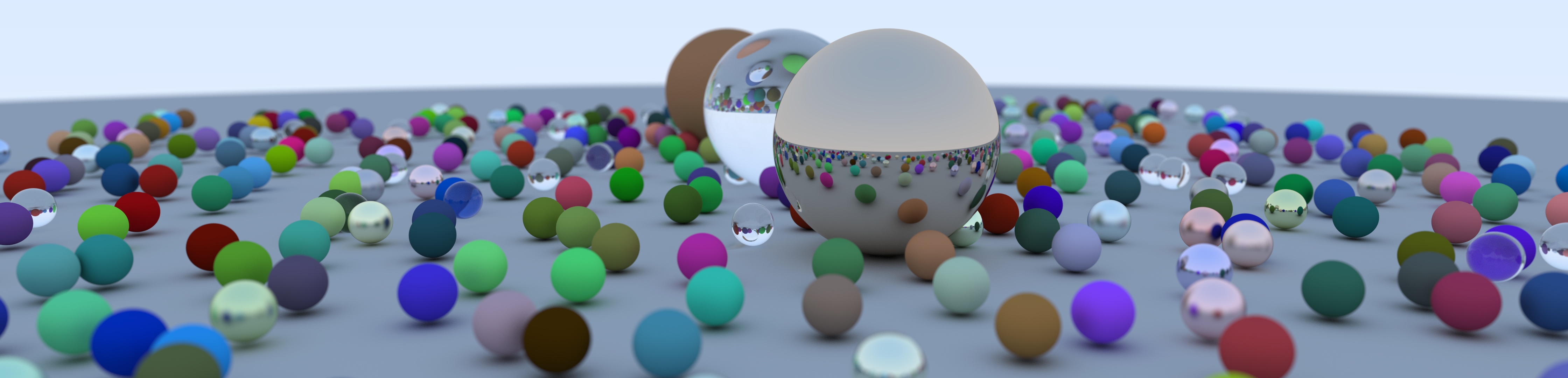
These two small changes give us a much closer result to the final image of “In One Weekend”. Rendering the scene in a resolution of 4480 x 1080 with 1k spp gives us:
Chapter 1 - Motion Blur
After this (very long) introduction, we are finally getting started with “The Next Week”. In the first chapter of his book, Peter Shirley introduces motion blur. He does that by storing at the ray the time it exists. We can do that by adding a float variable named ‘time’ to our prd.in structure, in the prd.h file.
We set the time the ray is generated at the color function of the raygen.cu shader:
//...
PerRayData prd;
prd.in.randState = &rnd;
prd.in.time = time0 + rnd() * (time1 - time0);
// ...
The camera will, basically, generate rays between the moments time0 and time1.
Finally, we add a moving sphere. Compared to the original sphere.cu file, we need to consider the fact that its center is now a function related to the time the ray hits the primitive and two different positions, the origin and destination of the sphere movement.
__device__ float3 center(float time) {
	return center0 + ((time - time0) / (time1 - time0)) * (center1 - center0);
}

// ...
float3 normal = (hit_rec_p - center(prd.in.time)) / radius;
// ...
The bounding box of this moving sphere is defined as:
RT_PROGRAM void get_bounds(int pid, float result[6]) {
    optix::Aabb* box0 = (optix::Aabb*)result;
    box0->m_min = center(time0) - radius;
    box0->m_max = center(time0) + radius;

    optix::Aabb box1;
    box1.m_min = center(time1) - radius;
    box1.m_max = center(time1) + radius;

    // extends box to include the t1 box
    box0->include(box1);
}
We should also update our CMakeLists.txt file to include our newly created external variable embedded_moving_sphere_programs and its correspondent file programs/hitables/moving_sphere.cu. This has to be done each time you add a new file to the project. The external variable should be declared in its correspondent header file.
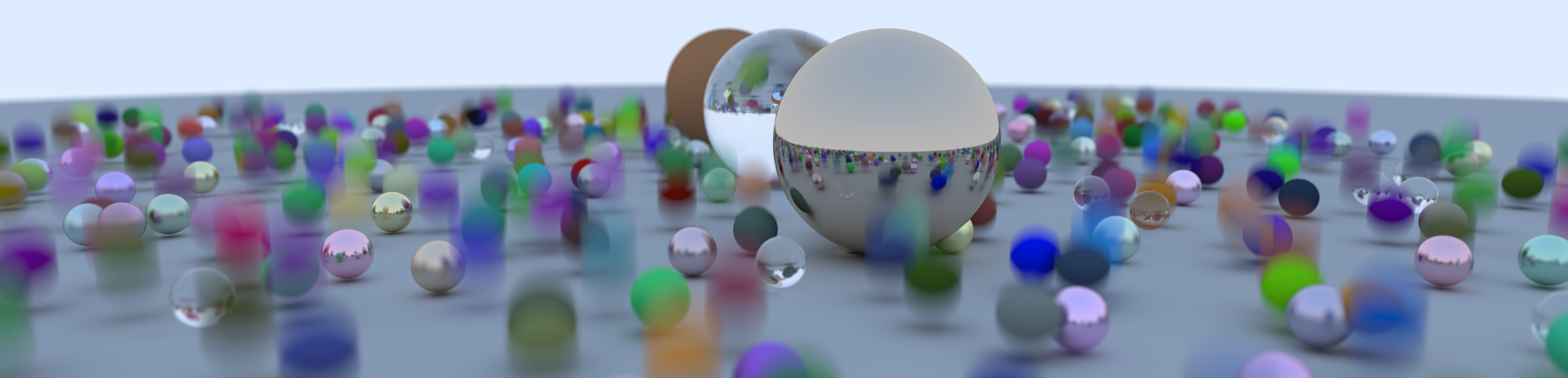
Rendering the scene in a resolution of 4480 x 1080 with 1k spp gives us:
Long after finishing this portion of the project I realized that OptiX has built-in functions related to motion blur at least since its 5.0 version. I eventually plan to come back to this and update the code to comply with that. The results should remain the same, though.
The code for this chapter is available here.
Chapter 2 - Bounding Volume Hierarchies
As mentioned before, one of the best things about using a ray tracing API like OptiX is the fact that it naturally supports state-of-the-art acceleration structures. While no extra code is needed here, I recommend the read of the documentation regarding this topic, where it’s described the pros and cons of using each one of the acceleration structures and some further info about how to properly build your node graph.
It’s also worth to note that, if for some reason you want to customize the way OptiX traverse your scene rather than using the traditional acceleration structures, you can make use of Selector nodes and Visit Programs.
Chapter 3 - Solid Textures
In the third chapter of “The Next Week”, Shirley introduces procedural textures, starting with constant and checkered textures. The best way I found to do something similar to that in OptiX was to use Callable Programs. Callable Programs are more flexible, considering they can take arguments and return values like other CUDA functions. In the device side, we may create a different .cu file for each texture callable program. For the constant texture, we have:
#define RT_USE_TEMPLATED_RTCALLABLEPROGRAM 1
#include <optix_world.h>

#include "../vec.h"

rtDeclareVariable(float3, color, , );

RT_CALLABLE_PROGRAM float3 sample_texture(float u, float v, float3 p) {
    return color;
}
with the checkered texture being implemented in an analogous way to its CPU counterpart. Then, we change the metal.cu and lambertian.cu material files to make use of sample_texture programs:
#define RT_USE_TEMPLATED_RTCALLABLEPROGRAM 1
#include <optix_world.h>
// ...
rtDeclareVariable(rtCallableProgramId<float3(float, float, float3)>, sample_texture, , );
// ...
attenuation = sample_texture(hit_rec_u, hit_rec_v, hit_rec_p);
Note that here we use bindless callable programs. You can also set bound callable programs to RTvariables as mentioned in the documentation.
On the host side, we create a new textures.h header with struct definitions for our newly created textures. The texture structs are similar to the already existing material ones, containing the needed parameters and an assignTo method. The assignTo method of the Constant_Texture is:
virtual optix::Program assignTo(optix::GeometryInstance gi, optix::Context &g_context) const override {
  optix::Program textProg = g_context->createProgramFromPTXString
                  (embedded_constant_texture_programs, "sample_texture");

  textProg["color"]->set3fv(&color.x);
  gi["sample_texture"]->setProgramId(textProg);

  return textProg;
}
with the Checker_Texture once again being analogous:
virtual optix::Program assignTo(optix::GeometryInstance gi, optix::Context &g_context) const override {
  optix::Program textProg = g_context->createProgramFromPTXString
              (embedded_checker_texture_programs, "sample_texture");

  /* this defines how the secondary texture programs will be named
  in the checkered program context. They might be named "sample_texture"
  in their own source code and context, but will be invoked by the names
  defined here. */
  textProg["odd"]->setProgramId(odd->assignTo(gi, g_context));
  textProg["even"]->setProgramId(even->assignTo(gi, g_context));

  /* this "replaces" the previous gi->setProgramId assigned to the geometry
  by the "odd" and "even" assignTo() calls. In practice, this assigns the
  actual checkered_program sample_texture to the material. */
  gi["sample_texture"]->setProgramId(textProg);

  return textProg;
}
Our Material structs are also slightly altered to take Texture objects, and properly assigning their callable programs, when applicable:
struct Lambertian : public Material {
  Lambertian(const Texture *t) : texture(t) {}

  /* create optix material, and assign mat and mat values to geom instance */
  virtual void assignTo(optix::GeometryInstance gi, optix::Context &g_context) const override {
    optix::Material mat = g_context->createMaterial();

    mat->setClosestHitProgram(0, g_context->createProgramFromPTXString
                              (embedded_lambertian_programs, "closest_hit"));

    gi->setMaterial(/*ray type:*/0, mat);
    texture->assignTo(gi, g_context);
  }
  const Texture* texture;
};
Before you attempt to compile the program, take note that, starting on CUDA 8.0, to be able to use Callable Programs you need to pass a –relocatable-device-code=true or -rdc flag to the NVCC compiler. In our CMake script, this can be done by editing the configure_optix.cmake file.
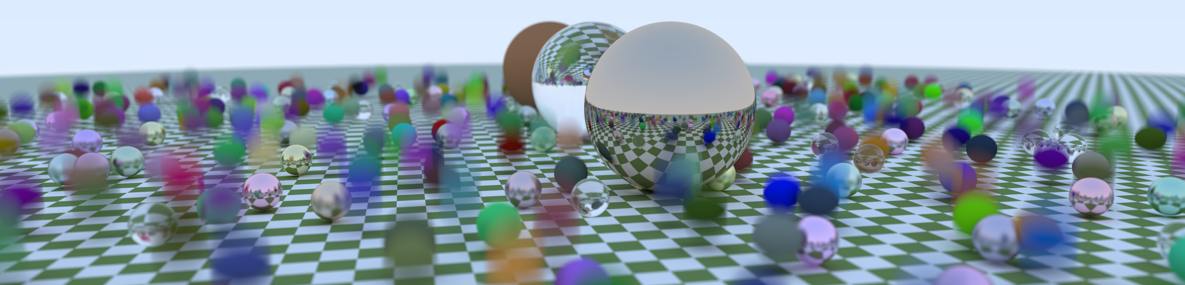
Rendering the scene in a resolution of 4480 x 1080 with 1k spp gives us:
The code for this chapter is available here.
Chapter 4 - Perlin Noise
For the Perlin Noise texture, we once again use callable programs. Overall, the only thing to note here is that we need to precompute the Perlin vectors and pass them to the device as OptiX input buffers. The device texture file noise_texture.cu is as follows:
// ...

rtDeclareVariable(float, scale, , );

// buffer definitions
rtBuffer<float3, 1> ranvec;
rtBuffer<int, 1> perm_x;
rtBuffer<int, 1> perm_y;
rtBuffer<int, 1> perm_z;

// ...

RT_CALLABLE_PROGRAM float3 sample_texture(float u, float v, float3 p) {
    return make_float3(1, 1, 1) * 0.5 * (1 + sin(scale * p.z + 5 * turb(scale * p)));
}
With the perlin_interp, noise and turb functions being roughly the same as in “The Next Week”. The assignTo method of the Noise_Texture struct is:
virtual optix::Program assignTo(optix::GeometryInstance gi, optix::Context &g_context) const override {
  optix::Buffer ranvec = g_context->createBuffer(RT_BUFFER_INPUT, RT_FORMAT_FLOAT3, 256);
  float3 *ranvec_map = static_cast<float3*>(ranvec->map());

  for (int i = 0; i < 256; ++i)
    ranvec_map[i] = unit_float3(-1 + 2 * rnd(), -1 + 2 * rnd(), -1 + 2 * rnd());
  ranvec->unmap();

  optix::Buffer perm_x, perm_y, perm_z;
  perlin_generate_perm(perm_x, g_context);
  perlin_generate_perm(perm_y, g_context);
  perlin_generate_perm(perm_z, g_context);

  optix::Program textProg = g_context->createProgramFromPTXString
                (embedded_noise_texture_programs, "sample_texture");

  textProg["ranvec"]->set(ranvec);
  textProg["perm_x"]->set(perm_x);
  textProg["perm_y"]->set(perm_y);
  textProg["perm_z"]->set(perm_z);
  textProg["scale"]->setFloat(scale);

  gi["sample_texture"]->setProgramId(textProg);

  return textProg;
}
with perlin_generate_perm being defined as:
void perlin_generate_perm(optix::Buffer &perm_buffer, optix::Context &g_context) const {
  perm_buffer = g_context->createBuffer(RT_BUFFER_INPUT, RT_FORMAT_INT, 256);
  int *perm_map = static_cast<int*>(perm_buffer->map());

  for (int i = 0; i < 256; i++)
    perm_map[i] = i;
  permute(perm_map);
  perm_buffer->unmap();
}
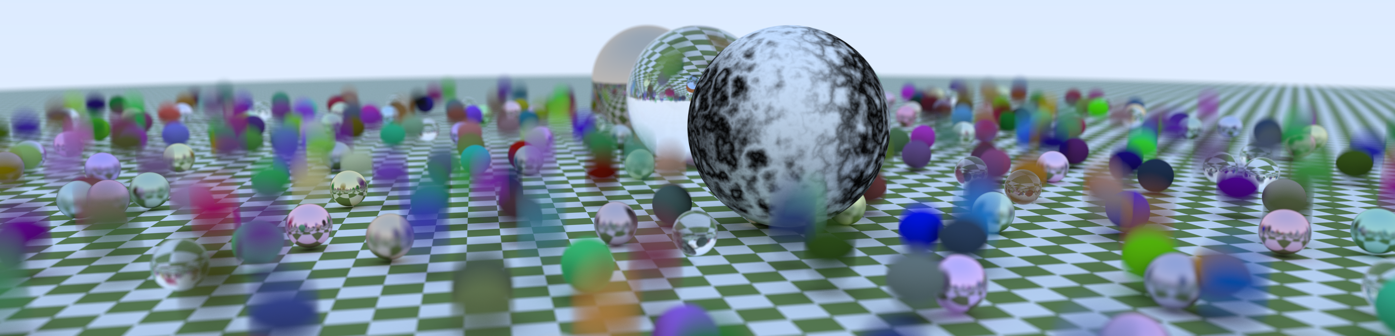
Finally, rendering the scene in a resolution of 4480 x 1080 with 1k spp gives us:
The code for this chapter is available here.
Chapter 5 - Image Texture Mapping
In the Chapter 5 of “The Next Week”, Shirley adds image textures to the project. This is done by loading a file with the same stbi library and sampling it with UV coordinates. We do something similar, also using the stbi loader, but with the help of texture samplers available on OptiX. The image_texture.cu callable program is:
// ...
rtTextureSampler<float4, 2> data;

RT_CALLABLE_PROGRAM float3 sample_texture(float u, float v, float3 p) {
    return make_float3(tex2D(data, u, v));
}
with the host method assignTo being defined as:
virtual optix::Program assignTo(optix::GeometryInstance gi, optix::Context &g_context) const override {
  optix::Program textProg = g_context->createProgramFromPTXString
                    (embedded_image_texture_programs, "sample_texture");

  textProg["data"]->setTextureSampler(loadTexture(g_context, fileName));

  gi["sample_texture"]->setProgramId(textProg);

  return textProg;
}
We do the actual image file load in the function loadTexture. We also define and configure the texture sampler there.
optix::TextureSampler loadTexture(optix::Context context, const std::string fileName) const {
  int nx, ny, nn;
  unsigned char *tex_data = stbi_load((char*)fileName.c_str(), &nx, &ny, &nn, 0);

  optix::TextureSampler sampler = context->createTextureSampler();
  sampler->setWrapMode(0, RT_WRAP_REPEAT);
  sampler->setWrapMode(1, RT_WRAP_REPEAT);
  sampler->setWrapMode(2, RT_WRAP_REPEAT);
  sampler->setIndexingMode(RT_TEXTURE_INDEX_NORMALIZED_COORDINATES);
  sampler->setReadMode(RT_TEXTURE_READ_NORMALIZED_FLOAT);
  sampler->setMaxAnisotropy(1.0f);
  sampler->setMipLevelCount(1u);
  sampler->setArraySize(1u);

  optix::Buffer buffer = context->createBuffer(RT_BUFFER_INPUT, RT_FORMAT_UNSIGNED_BYTE4, nx, ny);
  unsigned char * data = static_cast<unsigned char *>(buffer->map());

  for (int i = 0; i < nx; ++i) {
    for (int j = 0; j < ny; ++j) {
      int bindex = (j * nx + i) * 4;
      int iindex = ((ny - j - 1) * nx + i) * nn;

      data[bindex + 0] = tex_data[iindex + 0];
      data[bindex + 1] = tex_data[iindex + 1];
      data[bindex + 2] = tex_data[iindex + 2];

      if(nn == 4)
        data[bindex + 3] = tex_data[iindex + 3];
      else //3-channel images
        data[bindex + 3] = (unsigned char)255;
    }
  }

  buffer->unmap();
  sampler->setBuffer(buffer);
  sampler->setFilteringModes(RT_FILTER_LINEAR, RT_FILTER_LINEAR, RT_FILTER_NONE);
  return sampler;
}
Rendering the scene in a resolution of 4480 x 1080 with 1k spp gives us:
The code for this chapter is available here.
Chapter 6 - Rectangles & Lights
The Chapter 6 of “The Next Week” introduces Rectangles & Lights. Here, they are implemented mostly in an analogous way. The intersection function for the X-axis aligned rectangle in the aarect.cu file is given by:
RT_PROGRAM void hit_rect_X(int pid) {
    float t = (k - ray.origin.x) / ray.direction.x;
    if (t > ray.tmax || t < ray.tmin)
        return;

    float a = ray.origin.y + t * ray.direction.y;
    float b = ray.origin.z + t * ray.direction.z;
    if (a < a0 || a > a1 || b < b0 || b > b1)
        return;

    if (rtPotentialIntersection(t)) {
        hit_rec_p = ray.origin + t * ray.direction;

        // flip normal
        float3 normal = make_float3(1.f, 0.f, 0.f);
        if(0.f < dot(normal, ray.direction))
            normal = -normal;
        hit_rec_normal = normal;

        hit_rec_u = (a - a0) / (a1 - a0);
        hit_rec_v = (b - b0) / (b1 - b0);

        rtReportIntersection(0);
    }
}
The only thing to note here is how we handle the normal flipping. Differently from the book, where we needed to chain a flip_normal followed by a hitable, we can get a two sided rectangle by using the dot(normal, ray.direction) test. Another possibility was to use a boolean parameter ‘flip’ to check whether or not the normal should be flipped, giving you something close to what’s done by Shirley originally.
For the diffuse light, some changes are necessary in the per ray data, adding a float3 variable to our prd.out struct, representing the light emitted by the material of a geometry. Our closest_hit program in each of the materials become:
RT_PROGRAM void closest_hit() {
  prd.out.emitted = emitted();
  prd.out.scatterEvent
    = scatter(ray,
              *prd.in.randState,
              prd.out.scattered_origin,
              prd.out.scattered_direction,
              prd.out.attenuation)
    ? rayGotBounced
    : rayGotCancelled;
}
with the emitted() function being defined differently depending on your material. Non emissive materials can return make_float3(0.f) to represent the fact that no light is emitted. For the diffuse light, like the original book we make use of the texture assigned to our material, sampling it with the given u, v and p parameters. At the same time, its scatter function returns false:
inline __device__ bool scatter(const optix::Ray &ray_in,
                               DRand48 &rndState,
                               vec3f &scattered_origin,
                               vec3f &scattered_direction,
                               vec3f &attenuation) {
  return false;
}

inline __device__ float3 emitted(){
  return sample_texture(hit_rec_u, hit_rec_v, hit_rec_p);
}
Finally, we need to update our color function in the raygen.cu shader, to include the emitted light:
inline __device__ vec3f color(optix::Ray &ray, DRand48 &rnd) {
  PerRayData prd;
  prd.in.randState = &rnd;
  prd.in.time = time0 + rnd() * (time1 - time0);

  vec3f attenuation = 1.f;

  /* iterative version of recursion, up to depth 50 */
  for (int depth = 0; depth < 50; depth++) {
    rtTrace(world, ray, prd);
    if (prd.out.scatterEvent == rayDidntHitAnything){
      // ray got 'lost' to the environment - 'light' it with miss shader
      return attenuation * missColor(ray);
    }

    else if (prd.out.scatterEvent == rayGotCancelled)
      return attenuation * prd.out.emitted;

    else { // ray is still alive, and got properly bounced
      attenuation = prd.out.emitted + attenuation * prd.out.attenuation;
      ray = optix::make_Ray(/* origin   : */ prd.out.scattered_origin.as_float3(),
                            /* direction: */ prd.out.scattered_direction.as_float3(),
                            /* ray type : */ 0,
                            /* tmin     : */ 1e-3f,
                            /* tmax     : */ RT_DEFAULT_MAX);
    }
  }

  // recursion did not terminate - cancel it
  return vec3f(0.f);
}
Rendering the scene in a resolution of 4480 x 1080 with 1k spp gives us:
The code for this chapter is available here.
Chapter 7 - Instances
What’s done by using instances in “The Next Week”, meaning translation and rotations, will be done by using OptiX Transform nodes in our version. Before we proceed, let’s check an example of an OptiX scene graph, from the API’s programming guide.
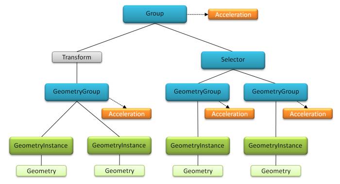
and this table showing which nodes can be children of other nodes, also from the programming guide:
| Parent node type | Child node types |
|---|---|
Geometry, Material and Acceleration |
none, these nodes can only be leafs |
GeometryInstance |
Geometry and Material |
GeometryGroup |
GeometryInstance and Acceleration |
Tranform and Selector |
GeometryGroup and Transform |
Group |
GeometryGroup, Transform and Acceleration |
Note that Transform nodes can only be children to Groups(and other Transform nodes). Until now, our root node was a GeometryGroup, but we can’t make it a parent of a Transform. In the scene.h header file, we should change how our scene graph is built. Considering that the camera parameters of the Cornell Box are different than the ones in the “One Weekend” scene, we want to move the camera setup to the creation function to keep our main file less cluttered. We also add a boolean ‘light’ parameter to our context, to be used in when our raygen.cu shader rays miss all the scene geometries.
optix::Group Cornell(optix::Context &g_context, Camera &camera, int Nx, int Ny) {
  optix::Group group = g_context->createGroup();
  group->setAcceleration(g_context->createAcceleration("Trbvh"));

  // ...

  addChild(createXRect(0.f, 555.f, 0.f, 555.f, 555.f, true, *green, g_context), group, g_context); // left wall
  addChild(createXRect(0.f, 555.f, 0.f, 555.f, 0.f, false, *red, g_context), group, g_context); // right wall
  addChild(createYRect(113.f, 443.f, 127.f, 432.f, 554.f, false, *light, g_context), group, g_context); // light
  addChild(createYRect(0.f, 555.f, 0.f, 555.f, 555.f, true, *white, g_context), group, g_context); // roof
  addChild(createYRect(0.f, 555.f, 0.f, 555.f, 0.f, false, *white, g_context), group, g_context); // ground
  addChild(createZRect(0.f, 555.f, 0.f, 555.f, 555.f, true, *white, g_context), group, g_context); // back walls
  addChild(createBox(vec3f(0.f), vec3f(165.f, 330.f, 165.f), *white, g_context), group, g_context); // big box
  addChild(createBox(vec3f(0.f), vec3f(165.f, 165.f, 165.f), *white, g_context), group, g_context); // small box

  // configure camera
  // ...
  camera = Camera(lookfrom, lookat, up, fovy, aspect, aperture, dist, 0.0, 1.0);

  // configure background color
  g_context["light"]->setInt(false);

  return group;
}
The other scene creation functions are changed in the same way. Our addChild function is defined as:
void addChild(optix::GeometryInstance gi, optix::Group &d_world, optix::Context &g_context){
  optix::GeometryGroup test = g_context->createGeometryGroup();
  test->setAcceleration(g_context->createAcceleration("Trbvh"));
  test->setChildCount(1);
  test->setChild(0, gi);

  int i = d_world->getChildCount();
  d_world->setChildCount(i + 1);
  d_world->setChild(i, test);
  d_world->getAcceleration()->markDirty();
}
Two other variations of this function should be defined in case its first parameter is a GeometryGroup or a Transform. GeometryGroups and Transforms can be assigned to a Group variable in the same way as it’s done above. For GeometryInstances, we need to create this new parent GeometryGroup because Groups can’t take them as children.
Now that we changed our scene graph, we can add Transforms to the scene. OptiX apply Transforms by using transformation matrices. As an example, our translate method and its transformation matrix are defined as:
optix::Matrix4x4 translateMatrix(vec3f offset){
  float floatM[16] = {
      1.0f, 0.0f, 0.0f, offset.x,
      0.0f, 1.0f, 0.0f, offset.y,
      0.0f, 0.0f, 1.0f, offset.z,
      0.0f, 0.0f, 0.0f, 1.0f
    };
  optix::Matrix4x4 mm(floatM);

  return mm;
}

optix::Transform translate(optix::GeometryInstance gi, vec3f& translate, optix::Context &g_context){
  optix::Matrix4x4 matrix = translateMatrix(translate);

  optix::GeometryGroup d_world = g_context->createGeometryGroup();
  d_world->setAcceleration(g_context->createAcceleration("Trbvh"));
  d_world->setChildCount(1);
  d_world->setChild(0, gi);

  optix::Transform translateTransform = g_context->createTransform();
  translateTransform->setChild(d_world);
  translateTransform->setMatrix(false, matrix.getData(), matrix.inverse().getData());

  return translateTransform;
}
The inverse of our Transforms matrix should be given as the third parameter of the setMatrix function as an optimization. Rotations are applied in the same way, and you can read more about 3D-rotation matrices here.
Last but not least, before attempting to render our scene, we should transform our geometry normal, with rtTransformNormal, and hit point, with rtTransformPoint, from the object space to the world space. This should be done in all intersection programs whose related geometry we plan to apply a transform. As an example:
float3 hit_point = ray.origin + t * ray.direction;
hit_point = rtTransformPoint(RT_OBJECT_TO_WORLD, hit_point);
hit_rec_p = hit_point;

float3 normal = make_float3(0.f, 0.f, 1.f);
hit_rec_normal = optix::normalize(rtTransformNormal(RT_OBJECT_TO_WORLD, normal));
Rendering the scene in a resolution of 4480 x 1080 with 1k spp gives us:

The code for this chapter is available here.
Chapter 8 - Volumes
The Volume chapter seemed a bit tricky to adapt to OptiX at first. I had to think about a way to intersect the boundary and the medium in the same GeometryInstance. Initially I tried to use AnyHit programs, but I quickly realized that wasn’t the best way to tackle this issue. As dhart mentions in the OptiX forums, ‘AnyHit shaders give you potentially out of order intersections for surfaces that you register with OptiX, which can be useful for visibility queries and some transparency effects and things like that, but they may not be the ideal mechanism for traversing your volume data.’ Further into the discussion, he suggested me to combine the boundary hit and the volume hit in the same intersection program, and that did the trick!
As it stands, I’m creating a hit_boundary device function for each geometry I want to use as a boundary. As an example, for the sphere:
inline __device__ bool hit_boundary(const float tmin, const float tmax, float &rec) {
  const float3 oc = ray.origin - center;

  // if the ray hits the sphere, the following equation has two roots:
  // tdot(B, B) + 2tdot(B,A-C) + dot(A-C,A-C) - R = 0

  // Using Bhaskara's Formula, we have:
  const float  a = dot(ray.direction, ray.direction);
  const float  b = dot(oc, ray.direction);
  const float  c = dot(oc, oc) - radius * radius;
  const float  discriminant = b * b - a * c;

  // if the discriminant is lower than zero, there's no real
  // solution and thus no hit
  if (discriminant < 0.f)
    return false;

  // first root of the sphere equation:
  float temp = (-b - sqrtf(discriminant)) / a;

  // if the first root was a hit,
  if (temp < tmax && temp > tmin) {
    rec = temp;
    return true;
  }

  // if the second root was a hit,
  temp = (-b + sqrtf(discriminant)) / a;
  if (temp < tmax && temp > tmin){
    rec = temp;
    return true;
  }

  return false;
}
These functions are, then, used in the volume intersection programs, like what happens in “The Next Week”:
RT_PROGRAM void hit_sphere(int pid) {
  float rec1, rec2;

  if(hit_boundary(-FLT_MAX, FLT_MAX, rec1))
    if(hit_boundary(rec1 + 0.0001, FLT_MAX, rec2)){
      if(rec1 < ray.tmin)
        rec1 = ray.tmin;

      if(rec2 > ray.tmax)
        rec2 = ray.tmax;

      if(rec1 >= rec2)
        return;

      if(rec1 < 0.f)
        rec1 = 0.f;

      float distance_inside_boundary = rec2 - rec1;
      distance_inside_boundary *= vec3f(ray.direction).length();

      float hit_distance = -(1.f / density) * log((*prd.in.randState)());
      float temp = rec1 + hit_distance / vec3f(ray.direction).length();

      if (rtPotentialIntersection(temp)) {
        float3 hit_point = ray.origin + temp * ray.direction;
        hit_point = rtTransformPoint(RT_OBJECT_TO_WORLD, hit_point);
        hit_rec_p = hit_point;

        float3 normal = make_float3(1.f, 0.f, 0.f);
        normal = optix::normalize(rtTransformNormal(RT_OBJECT_TO_WORLD, normal));
        hit_rec_normal = normal;

        hit_rec_u = 0.f;
        hit_rec_v = 0.f;

        rtReportIntersection(0);
      }
    }
}
Considering we already have these primitives working as independent geometries this might sound like extra work, but it’s the best (and easiest) way I managed to found to get the work done for now. If you manage to have a simpler idea, I would be glad to hear it!
For the volume boxes, rather than using the rectangle hit functions previously introduced by the book, I use a hit_boundary intersection function based on the slabs method from the Chapter 2’s BVH. It’s still a box, but as a single entity rather than several underlying primitives, in my opinion making it easier on OptiX to detect whether a ray hit any of its faces or not.
Rendering the scene in a resolution of 4480 x 1080 with 1k spp gives us:

You might notice that the boxes look considerably different then the ones from “The Next Week”, especially when you look at their bottom faces. I think this might be because I use a different intersection method here, but I’m not completely sure.
The code for this chapter is available here.
Chapter 9 - Final Scene
One thing I realized while trying to render the final scene with a high number of samples is the fact that my implementation was timing out. That was not exactly a bug. As NVIDIA’s Roger Allen mentions in this post, Windows has a GPU timeout detection of 5 to 10 seconds by default. If your OptiX program runs any longer than that, the system will give you an error message and abort the application, resulting in an exception. It’s not recommended to turn the timeout detection off, as that may lead to serious issues and system crashes when your GPU is in real trouble. Unless you have a second GPU that you can dedicate exclusively to rendering tasks, the usual approach is to do less work with a single kernel execution.
As I only have a single GPU, my general idea was to trace one ray per pixel per launch. Basically, our program launch in main.cpp becomes:
for(int i = 0; i < samples; i++){
    g_context["run"]->setInt(i);
    renderFrame(Nx, Ny);
    printf("Progress: %2f%%\r", (i * 100.f / samples));
}
Meanwhile, the renderPixel function of the raygen.cu shader becomes:
RT_PROGRAM void renderPixel() {
  DRand48 rnd;

  if(run == 0) {
    unsigned int init_index = pixelID.y * launchDim.x + pixelID.x;
    rnd.init(init_index);
  }
  else{
    rnd.init(seed[pixelID]);
  }

  vec3f col(0.f);

  if(run == 0)
    fb[pixelID] = col.as_float3();

  float u = float(pixelID.x + rnd()) / float(launchDim.x);
  float v = float(pixelID.y + rnd()) / float(launchDim.y);

  // trace ray
  optix::Ray ray = Camera::generateRay(u, v, rnd);

  // accumulate color
  col += color(ray, rnd);

  fb[pixelID] += col.as_float3();
  seed[pixelID] = rnd.state; // save RND state
}
For that approach to work we need to keep the RNG state on a seed buffer and use it on the samples to follow. We create the seed buffer on the host side, once again on main.cpp:
optix::Buffer createSeedBuffer(int Nx, int Ny) {
  optix::Buffer pixelBuffer = g_context->createBuffer(RT_BUFFER_OUTPUT);
  pixelBuffer->setFormat(RT_FORMAT_UNSIGNED_INT);
  pixelBuffer->setSize(Nx, Ny);
  return pixelBuffer;
}

// [...]

// Create a rng seed buffer
optix::Buffer seed = createSeedBuffer(Nx, Ny);
g_context["seed"]->set(seed);
I also changed the RNG device class from Ingo Wald’s implementation, adapting a XorShift32 version suggested by Aras Pranckevicius. The OptiX API has no support to doubles or longs, so using 32-bit unsigned ints seemed like a better idea here, considering I have to save the states on a buffer. I’m not completely sure, but it might be faster as well(GPUs behave better with single precision numbers).
// get the next 'random' number in the sequence
inline __device__ float operator() () {
  unsigned int x = state;

  x ^= x << 13;
  x ^= x >> 17;
  x ^= x << 15;

  state = x;

  return (x & 0xFFFFFF) / 16777216.0f;
}
Keep in mind that unsigned numbers don’t overflow, so you there’s no need to check that. Last but not least, we should average the frame buffer values, as well as applying gamma correction, in the host side before saving it to a file:
for (int j = Ny - 1; j >= 0; j--)
  for (int i = 0; i < Nx; i++) {
    int col_index = Nx * j + i;
    int pixel_index = (Ny - j - 1) * 3 * Nx + 3 * i;

    // average matrix of samples
    vec3f col = cols[col_index] / float(samples);

    // gamma correction
    col = vec3f(sqrt(col.x), sqrt(col.y), sqrt(col.z));

    // from float to RGB [0, 255]
    arr[pixel_index + 0] = int(255.99 * clamp(col.x)); // R
    arr[pixel_index + 1] = int(255.99 * clamp(col.y)); // G
    arr[pixel_index + 2] = int(255.99 * clamp(col.z)); // B
  }
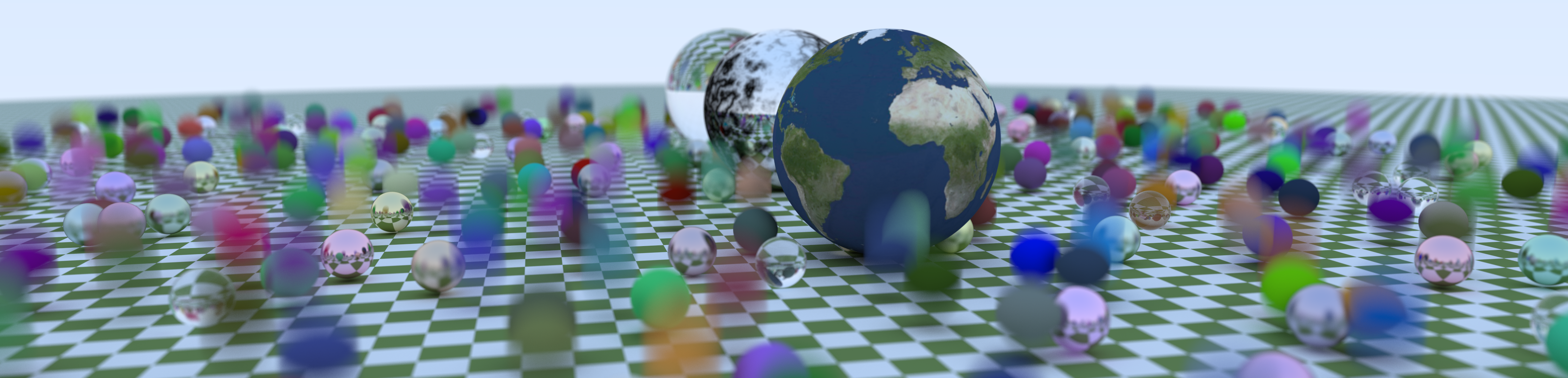
And that’s it! Now our Path Tracer is ready to scale to several thousand samples. Rendering the final scene in 4480x1080 pixels with 10k spp gives us the first image of this post:
The code for this chapter is available here.
Next Steps, Further Reading & Final Remarks
And we are done with “The Next Week” in OptiX! The post was way longer than I initially intended, but I hope I somehow managed to help people trying to get into GPU ray tracing with the NVIDIA API. I will expand the project right away to port the third book, “The Rest of Your Life”, to OptiX as well. Once again I plan to blog about it when I’m done.
If you want to learn more about OptiX programming, I recommend reading the GTC introduction presentations(here and here), as well as watching the record of its 2018 edition where NVIDIA’s Detlef Roettger explains each project of the OptiX Advanced Samples repository. The OptiX Quickstart tutorial and the SDK samples, found in the OptiX SDK installation folder, are also a great place to start. Last but not least, don’t forget to check the OptiX Developer Forums.
For more info about CUDA programming, this blog post by Roger Allen that I previously linked is a great way to start. He talks about his CUDA version of “In One Weekend” as well as linking even further materials. That was my first contact with CUDA and GPU programming at all. I went through his blog post and implementation to learn some more about the language and its intrinsics, about which Allen goes in detail, before attempting to implement this OptiX project. Allowing concurrency and taking (extra) care with memory management in GPU programming are two of the most important things I was able to take from that. Soon, I began to realize some things were considerably harder to do in CUDA than in traditional C++ code. As it happens in OptiX, it’s a completely different paradigm, as you have to think about both the device and host sides. It’s, arguably, already easy to get lost with pointers in traditional C++ code, which means you need to take even greater care here. Making a BVH work properly in pure CUDA code, for example, turned out not to be an easy task.
As I mentioned before, I’m just getting started myself, both with OptiX and the Graphics field as a whole, so this project and the post itself are bound to have errors. Once again, if you find any mistakes or typoes, if you have critics or suggestions, or any kind of feedback at all, really, I would be glad to hear it. Just let me know through Twitter or in the comments section below.
Huge thanks for reading! I really appreciate it.